Cme index bitcoin
Contents:
JB , the Jarque-Bera test statistic for normality. LB 2 12 denote the Ljung-Box Q test statistic for return squares up to lag order The following section is taken from Shi et al. We can write an unrestricted VAR p in multi-variate regression format simply as:. In order to test the null hypothesis that y 2 t does not Granger cause y 1 t , the Wald test for such restrictions can be denoted as:. Each row picks one of the coefficients to set to zero under the non-causal null hypothesis.
There are p coefficients on the lagged values of y 2 t in Eq. Following the recent bubble detection tests of Phillips, Shi, and Yu [] , Shi et al. If the Wald statistic sequence exceeds its corresponding critical value, a significant change in causality is detected.
The origination termination date of a change in causality is identified as the first observation whose test statistic value exceeds goes below its corresponding critical values. This is known as the recursive evolving procedure. Let f e and f f denote the origination and termination points in the causal relationship, which are estimated as the first chronological observation whose test statistic respectively exceeds or falls below the critical value.
Suggested Comparisons
The dating rules of the rolling and recursive evolving algorithms are given as:. For multiple switches, the origination and termination dates are calculated in a similar fashion. As Shi et al. Hence, we investigate the potential causal relationship using these two procedures in this paper. The minimum window size f 0 is set to 0. The critical values are obtained from a bootstrapping procedure with replications.
Following Stock and Watson [] and Hasbrouck [] , Eq. This term is the major focus of different information share measures. In Hasbrouck [] , all the prices are equal in equilibrium because these series correspond to the prices of the same security being traded in multiple markets. Thus, Eq. It can be decomposed as:. The first last represents the contribution to the common factor innovation from the first last market [ Baillie et al. When the covariance matrix is not diagonal, that is, the innovations are not independent, the IS of market j is given by Hasbrouck [] ,.
This is known as the ordering problem where the calculation of IS using Eq. Thus the IS measure of any market is not unique. Lien and Shrestha [] propose a new measure of information share to resolve the ordering problem of the Hasbrouck information share. The new measurement is called generalised modified information share GIS. GIS utilises a different factor structure that is based upon the correlation matrix of innovations instead of the covariance matrix.
However, this assumption is restrictive since the one-to-one cointegrating relationship does not necessarily hold in the real world. Therefore, such new measure can apply to series that do not have the one-to-one cointegrating relationships between them. When the innovations are independent, the variance of long-run impact on the i th series is:. The contribution of the innovation of series j to the total variance of the common factor of series i is then represented by:.
S j , i G is so called generalised information share GIS of series j which is independent of i. When the innovations are not independent, the GIS of series j can be calculated as:. It should be noted that the GIS measure uses the factor structure same as the MIS; thus it would also be independent of the ordering problem. We assume that error correction coefficients in Eq. Let S t and F t be the natural logarithms of daily prices of the spot and futures contacts, respectively.
Bybit Climbs Past CME to Become Second-Largest Bitcoin Futures Exchange
If the two series are integrated at the same order, a potential cointegration relationship where the cointegrating coefficient is time variant rather than static, is represented as:. Therefore, Eq. Park and Hahn [] employ the superfluous regression approach to test the null hypothesis of the time-varying coefficient cointegration against the alternative of the spurious regression with non-stationary innovations. The corresponding test statistic is defined as:. In this paper, following the literature, we choose s to be 4. In addition, we choose k from a range between 1 and 5.
The optimal k is picked based on the adjusted R-square of CCR. The test statistic follows a Chi-square distribution with degree of freedom equal to the number of restrictions. It should be noted that the conditional variance-covariance matrix underlie the calculation of time-varying information share measures. Most of the applications of BGARCH models for estimating the optimal hedge ratio assume that the error terms follow a bivariate conditional normal distribution. Typical distributional features of financial time-series data are excess kurtosis and asymmetry.
In this paper, we employ a semi-nonparametric SNP approach to address the issue of excess kurtosis and non-zero skewness in the marginal return distribution.
- low fee btc wallet?
- bitcoin is forking.
- microsoft bitcoin exchange.
- best paypal bitcoin exchange!
- How To Invest In Bitcoin Futures.
In particular, a two-step estimation procedure is applied to obtaining estimates for the individual GARCH processes, conditional correlation matrix and marginal skewness and kurtosis parameters. First, the individual conditional variance equations are estimated via QMLE assuming Gaussian distribution and standardised innovations are obtained.
Trade Bitcoin Futures
Second, the parameters that capture the conditional correlation and other higher order moments are obtained via the log-likelihood maximization over the whole sample. The log-likelihood of the multivariate SNP density that each observation at time t contributes to, without unnecessary constant components, is shown as:. R t is conditional correlation matrix defined by Eq.
The procedure does not require pre-filtering the data but it require the maximum order of integration for the VAR. Using several unit root tests to check the stationarity of log futures and spot prices, we conclude that all variables are I 1. The time-varying Wald test statistics for causal effects from Bitcoin spot prices to CBOE futures prices along with their bootstrapped critical values are shown in Fig.
The two rows illustrate the sequences of test statistics obtained from the rolling window and recursive evolving procedures respectively, while the columns of the figure refer to the two different assumptions for the residual error term homoskedasticity and heteroskedasticity for the VAR. Sequences of the test statistics start from April Under different model and error assumptions presented in Fig.
As a result, date-stamping results from Figs. The result suggests that the CBOE spot market may not be able to lead the futures market since the former responds to new information more slowly than the latter. We can see that, first, there is little evidence of Granger causality episodes based on the rolling window procedure as presented in Fig.
Second, the recursive evolving approach offers some different results.
As shown in Fig. As a result, the null hypothesis of no Granger causality can be rejected. Similarly, under the error assumption of heteroscedasticity, Fig. As noted in Shi et al.
- steem btc market?
- cross chain bitcoin.
- contratos de futuros de btc.
- Bitcoin futures on the world’s biggest derivatives exchange signal the boom isn’t over yet.
- Bitcoin Futures - .
Next, therefore, we undertake our analysis using the CME futures prices and CME BRR to explore the causal relationship between futures and spot markets with the results presented as in Fig. For example, when we look at the date-stamping outcomes in Fig. When the recursive evolving procedure is applied as in Fig.
Finally, we conduct an analysis of Granger causality running from the CME futures to spot prices. Interestingly, we obtain significant evidence to reject the null of no Granger causality from the CME futures to spot prices as presented in Fig. The rolling window approach finds an episode of Granger causality between April and March in Fig. What is even more interesting is that the recursive evolving approach identifies an episode of Granger causality for the whole period between April and July as shown in Fig.
It is clear that our results are robust to different error assumptions. As the recursive evolving approach has higher power over the rolling window approach, we prefer the results obtained from the recursive evolving approach. Our results, therefore, suggest that the CME futures prices lead spot prices in the short term within the context of time-varying Granger causality.
Our result suggests there exists bi-directional Granger causality between the CME Bitcoin spot and futures prices. More importantly, given the duration of the Granger-causal episodes and the magnitude of the test statistics in Fig. From this we conclude that Granger causality runs from the futures market to the spot market.
This result further suggests that the CME Bitcoin futures market leads the spot since the former embeds the new information faster than the latter. The results from time-varying Granger causality tests present some very important findings. There are no Granger causality episodes running from the Gemini auction price spot prices to the CBOE futures prices;. The rolling window approach detects an episode April —March and recursive evolving approach detects an episode April —July running from the CME futures prices to spot prices;. There is bi-directional causal relationship between spot price and the CME futures prices;.
Compared with duration of causal episodes and the magnitude of the test statistics in Fig. Overall, our result show that there is unidirectional Granger causality running from the CBOE Bitcoin futures to spot markets, whereas there is bidirectional Granger causality between the CME Bitcoin futures and spot prices.
It should be noted that even though Granger bidirectionality cannot be rejected, the Granger causality from the futures to spot is stronger than the other way around which suggests that the Bitcoin futures market dominates the spot in terms of strength of the lead-lag responses. Our results enrich the literature by identifying the evolving Granger causality relations between two major Bitcoin futures markets and their spot assets where both futures markets play a leading role in the dynamic Granger causality processes.
The result is in line with prior studies on traditional financial futures markets that indicate futures market lead the spot in the between-market interactive processes see, e. Next we use Park and Hann's [] procedure to test for the existence of cointegration which allows for the possibility of estimating a time-varying cointegrating coefficient. Via the Engle-Granger Theorem we know that cointegration implies Granger causality in at least one direction such that non-rejection of cointegration strengthens any causality results represented above, although the theorem does not itself identify the direction of Granger causality.
Upon the non-rejection of non-static cointegration, that is, a time varying equilibrium when cointegrated time series hold, a dynamic error correction process between them is identified.
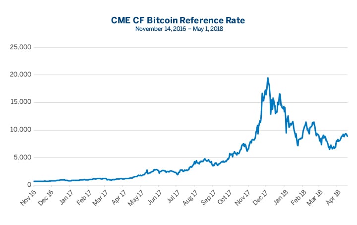
CME CF Bitcoin. CME CF Ether-Dollar.
This further reinforces the accuracy and robustness of the results of price discovery given the more accurate estimation of error correction coefficients. We also present the movements of the time-varying cointegration coefficients between the futures and spot markets in Fig. We, therefore, prefer the time-varying cointegration model rather than the time-invariant cointegration model. The Park Park and Hahn [] test results presented in Table 4 clearly show i that the null hypothesis that the cointegration specification, assuming a static cointegration relationship is statistically rejected, whereas ii the null hypothesis that the cointegration specification with a time-varying cointegration coefficient, governed by a FFF function of time, is not rejected at any conventional level.
The results hold for both futures markets.
Our results therefore suggest that time variations in the cointegration coefficients exists, which has implications for the long-run equilibrium between spot and futures prices. Moreover, in Table 4 the null hypothesis that all the coefficients in the FFF time function are jointly zero is rejected, again for both of the futures markets, again supporting the results in terms of time variations of the cointegration coefficients. Finally, we test three null hypotheses based on values of the variances of the cointegration coefficients. For the CBOE Bitcoin spot and futures markets, we test the null hypotheses that the variance equals 3.
Note that the sample variance equals 3. The test result shows that the first null is rejected, whereas the null hypothesis that variance equals 3. These results suggest that the variance of the cointegration coefficient for the CBOE Bitcoin spot and futures is not zero, supporting time variability of that coefficient. For the CME Bitcoin spot and futures markets, we test the null hypotheses that the variances equal 2. Test results show that the nulls that the variance equals 2. These results suggest that the variance of the cointegration coefficient for the CME Bitcoin spot and futures is not zero, again supporting time variability of the coefficient.
Overall, time variations in the cointegration coefficients are observed, substantiating a dynamic cointegrating model for the long-run relationship between Bitcoin spot and futures markets. This table presents results of Park and Hahn [] test. Results for the static time-invariant price discovery measures are summarized in Table 5. It should be pointed out that the CBOE futures market dominates the price discovery process. It is clear that the IS upper bound, lower bound and mid-point and GIS measures of the CME futures are higher than those of spot markets, indicating that the CME futures market outperforms in terms of static information shares price discovery.
This finding is consistent with the results of the time-varying Granger causality approaches reported in Section 4. The static time-invariant estimates of price discovery measure for Bitcoin spot and two futures markets. Results of the time-varying price discovery measures are summarized in Table 6. As can be seen from Panel A, the mean, maximum and minimum estimates of upper bound, lower bound and mid-point of the IS measures for the CME futures are higher than those of spot markets.
Similarly, the CBOE futures market outperforms the spot market in terms of conditional information shares as the mean, maximum and minimum estimates of upper bound, lower bound and mid-point of the IS measures for the CBOE futures market are also higher than those of the spot market. Hence, the conditional IS measures suggest that price discovery mainly takes place in the Bitcoin futures markets, rather than spot counterpart.
The results are consistent with static measures. In addition, standard deviations of the IS measures for the spot and futures markets are small, indicating that those measures are stable over the entire sample period.