Bitcoin and bubbles

Crypto Long & Short: No, Bitcoin Is Not in a Bubble

---

Consequently, given any European-type contingent claim, it is not possible in general to find a self-financing strategy whose terminal value exactly replicates the payoff of the claim. We recall that the notion of completeness is related to the uniqueness of the martingale measure. Indeed, in complete markets, the no-arbitrage price of any derivative is uniquely determined by the unique martingale measure.

Filter by Topic

One simple example of a candidate equivalent martingale measure is the so-called minimal martingale measure see [ 17 , 18 ] , which minimizes the relative entropy, of the objective measure P , with respect to any risk-neutral measure. In this setting, its economic interpretation is that agents do not wish to be compensated for the risk associated with the fluctuations of the stochastic attention factor, which corresponds to the hypothesis of [ 19 ] in the stochastic volatility framework.

Remark 3. Indeed, the authors only referred to a risk-neutral framework without describing the dynamics under the physical measure and consequently characterizing the existence of any equivalent martingale measure. Now, we compute the fair price of a Bitcoin European call option via the risk-neutral evaluation approach, so it can be expressed as expected value of the terminal payoff under the selected pricing measure, that is, the minimal martingale measure.

Here, N stands for the standard Gaussian cumulative distribution function, that is,. The proof is straightforward and may be derived by using similar arguments to those developed in [ 19 ]. Proposition 3. The risk-neutral price C t at time t of a European call option written on the Bitcoin with price S expiring in T and with strike price K is given by the formula. In order to appreciate the performance of the pricing formula in Eq.

Best overall pricing values are obtained when market attention is measured by volume; in the case of the SVI Google index, near-term options are very close to the mid-value of the bid-ask, while next-term options are overpriced. Comparison between model prices computed according to formula in Eq. Motivated by empirical evidences see for example [ 21 , 22 ] , we discuss a generalization of the model introduced in Section 3. Without loss of generality, we assume that the interest rate is fixed and equal to zero. In this setting, the discounted Bitcoin price trend and the market attention factor dynamics are described by.

The aim is to investigate the existence of asset-price bubbles in the underlying Bitcoin market model. By simulating trajectories for the asset price S according to the model in Eq. The mathematical theory of financial bubbles is developed, among others, in [ 23 , 24 , 25 ].

The case for believers

Precisely, we introduce the following definition from [ 23 ]. Definition 4. The Bitcoin price process S has a bubble on the time interval 0 T if S is a strict F -local martingale under the chosen risk-neutral measure. The term strict F -local martingale refers to the fact that S is an F -local martingale, but not a true F -martingale under the chosen risk-neutral measure.

Further, since S is nonnegative, we must have that S is an F -supermartingale we refer to [ 26 ] for rigorous definitions and related concepts. Remark 4. Note that stock bubbles arise if S has an equivalent local martingale measure but not an equivalent martingale measure. Arbitrage appears only if no equivalent local martingale measure exists. The local martingale property of the discounted Bitcoin price process S under Q implies the following condition:.

We have the following result, which allows to detect the presence of bubbles in this setting. Proposition 4. In the model outlined in Eq. Precisely, it is possible to show that the martingale property of the discounted stock price S under Q 0 , given in Eq. Hence, a bubble arises if and only if the correlation parameter between stock returns and market attention is positive. Let us generalize the model introduced in Eq. We get. Analogous results as those in Section 2 can be derived by similar computations, and model parameters, for a fixed delay, can be estimated by means of the maximum likelihood method.

In order to estimate the delay parameter, we maximize the profile likelihood as defined in [ 15 ]. Details of this procedure can be found in [ 10 ]. The estimation results of model in Eq. Parameter estimates for model in Eq. In Figure 3 , we plot simulated trajectories of the price process in Eq. The different delays result in a shift to the south-east between the faster and slower reacting trajectories; in the picture, this behavior is sharp since the other model parameters are kept constant. By looking at the picture, the idea to model the price of Bitcoin in different exchanges by the same model in Eq.

Note that within this model, prices for Bitcoin traded in different exchanges are perfectly correlated.

Indeed, this is what happens in observed data; considering daily prices from January to June for Bitstamp, Kraken, Cex. We fit model in Eq. Model fitting with delay parameter: outcomes for Bitstamp and Gdax exchanges when attention is measured by the trading volume. Model fitting with delay parameter: outcomes for Bitstamp and Gdax exchanges when attention is measured by the SVI index. It is evident from the outcomes in Table 4 that the model parameters are not significantly different while the delay might be quite different as if the reaction to the attention factor is faster for some exchanges and slower for others.

However, environmental impact is something that we should all be concerned about. It is important to distinguish digital currencies and blockchain technology, the distributed ledger that records bitcoin transactions. Even if one does not like crypto currencies, there is no doubt that blockchain technology created a new and important area of innovation.

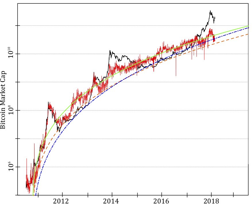
As with many other areas, the companies that use blockchain to work on not-very-glamorous things such as improving container shipping documentations may create lasting value using this technology. Aleh Tsyvinski Arthur M. Okun Professor of Economics. Why is bitcoin still going up? These results are found to be robust with regards to the chosen fitting window. Comparing Bitcoin market cap black line with predicted market cap based on various generalized Metcalfe regressions of active users.

The remaining lines plug smoothed active users non-parametric up to and the nonlinear regression starting in to project beyond into the generalized Metcalfe formula with different parameters: the smooth green line for the estimated coefficients 1. The lower inset plot with grey line is the price per bitcoin in USD. On this basis alone, the current market looks similar to that of early , which was followed by a year of sideways and downward movement.

Associated Data

Some separate fundamental development would need to exist to justify such high valuation, which we are unaware of. Using the generalized Metcalfe regression onto smoothed active users as well as its support lines, one can identify in figure 2 four main bubbles corresponding to the largest upward deviations of the market cap from this estimated fundamental value. These four bubbles in market cap are highlighted in figure 3 , and detailed in table 1 —in some cases exhibiting a fold increase in less than six months!

In all cases, the burst of the bubble is attributed to fundamental events, listed below, in particular for the first three bubbles, which corrected rapidly at the time of the clearly relevant news. The fourth and very recent bubble was much longer, and it is plausible that the main news there was really the 20 USD value of Bitcoin, i. Upper triangle: market cap of Bitcoin with four major bubbles indicated by bold coloured lines, numbered, and with bursting date given.

Lower triangle: the four bubbles scaled to have the same log-height and length, with the same colour coding as the upper, and with pure hyperbolic power law and LPPLS models fitted to the average of the four scaled bubbles, given in dashed and solid black, respectively. Bubble statistics. The bubbles correspond to the numbering in figure 3.

Is Bitcoin in a Dangerous Bubble?

Bubble 5 corresponds to approximately the last six months of the fourth bubble, and will be used in the next section. The price data for Bitcoin is from Bitstamp, in USD, hourly from 1 January to 8 January ; the Bitcoin circulating supply comes from blockchain. Of particular interest here is that, although the height and length of the bubbles vary considerably, when scaled to have the same log-height and length, a near-universal super-exponential growth is evident, as diagnosed by the overall upward curvature in this linear-logarithmic plot lower figure 3.

And in this sense, like a sandpile, once the scaled bubble becomes steep enough angle of repose , it will avalanche, while the precise triggering nudge is essentially irrelevant.

Navigation menu

Gox closes. T 1 is the starting time, and t c the stopping or the so-called critical time by which the bubble must burst. The window T 1 , T 2 needs to be specified, with selection of the start of the bubble T 1 often being less obvious. In this case, generalized least squares GLS provides a conventional solution, which has been used with LPPLS [ 45 — 47 ] and, if well specified, has optimal properties. Here, we opt for a simple specification of the error model, being auto-regressive of order 1, Here, we focus on t c , the critical time at which the bubble is most likely to burst.

No, Bitcoin Is Not in a Bubble - CoinDesk

The sample is taken at equidistant points. Given our proposed fundamental value of Bitcoin based on the generalized Metcalfe regressions presented above, we define the Market-to-Metcalfe value MMV ratio. In particular, the parameters of the hyperbolic power-law and LPPLS models fitted on the MMV ratio data, for the full bubble lengths, are given in table 4.

• mine bitcoin chrome
• bitcoin insanity coupon
• meetup bitcoin zurich
• bitcoin future trading
• bitcoin why use it
• algorithm bitcoin trading
• iota price prediction bitcointalk